How LLMs Work - For The Rest Of Us

LLMs are fascinating. I’ve been using them for a while now, and it still surprises me that something like this actually works at all. And after spending time learning how they actually work, I ended up even more surprised.

In this blog, I will try to explain how LLMs work without using much math, although some basic understanding of a vector will help relate more. We will take one example and carry it across the article to understand all the different parts. When I type:

The capital of France is

and the model responds with Paris, what actually happens? Is it searching some database? Or running a very large if/else tree that someone wrote?

You probably already know that’s not what is happening. An LLM is not normal application logic. There is no giant handwritten rulebook inside the model doing something like:

if prompt asks "capital of France":
  return "Paris"

Instead, an LLM turns text into token vectors, repeatedly enriches those vectors through transformer layers, and then uses the final vector of the last token to score the next token.

We will go through each of these steps one by one.

In this article I will describe a classic, simplified version of a transformer. Real models, especially newer ones, tweak plenty of internal details. The big picture still holds, just note that not everything described in the article applies exactly to every model.

Table of Contents

• Text Becomes Tokens
• What Is A Vector Here?
• The Transformer
• How Attention Works
• How Feed-Forward Works
• Features, Signals, And Patterns
• The Causal Mask
• Predicting The Next Token
• Why It Can Be Wrong
• Why Doesn’t It Always Pick The Best Match?
• Where Does Thinking Fit In?
• What About KV Cache?
• The Full Flow

Text Becomes Tokens

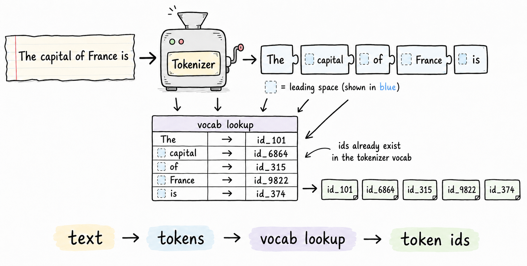
The model doesn’t read our prompt the way we do. The first step is tokenization, where the text is broken into small chunks called tokens. A token is sometimes a full word, sometimes a piece of a word, and sometimes a space, a punctuation mark, a code symbol, or a part of a JSON key.

For our prompt, the tokens may roughly look like this:

"The"
" capital"
" of"
" France"
" is"

The space before a word can be part of the token, so "capital" and " capital" may be two different tokens. Also, the model does not directly work with these words. It works with token ids.

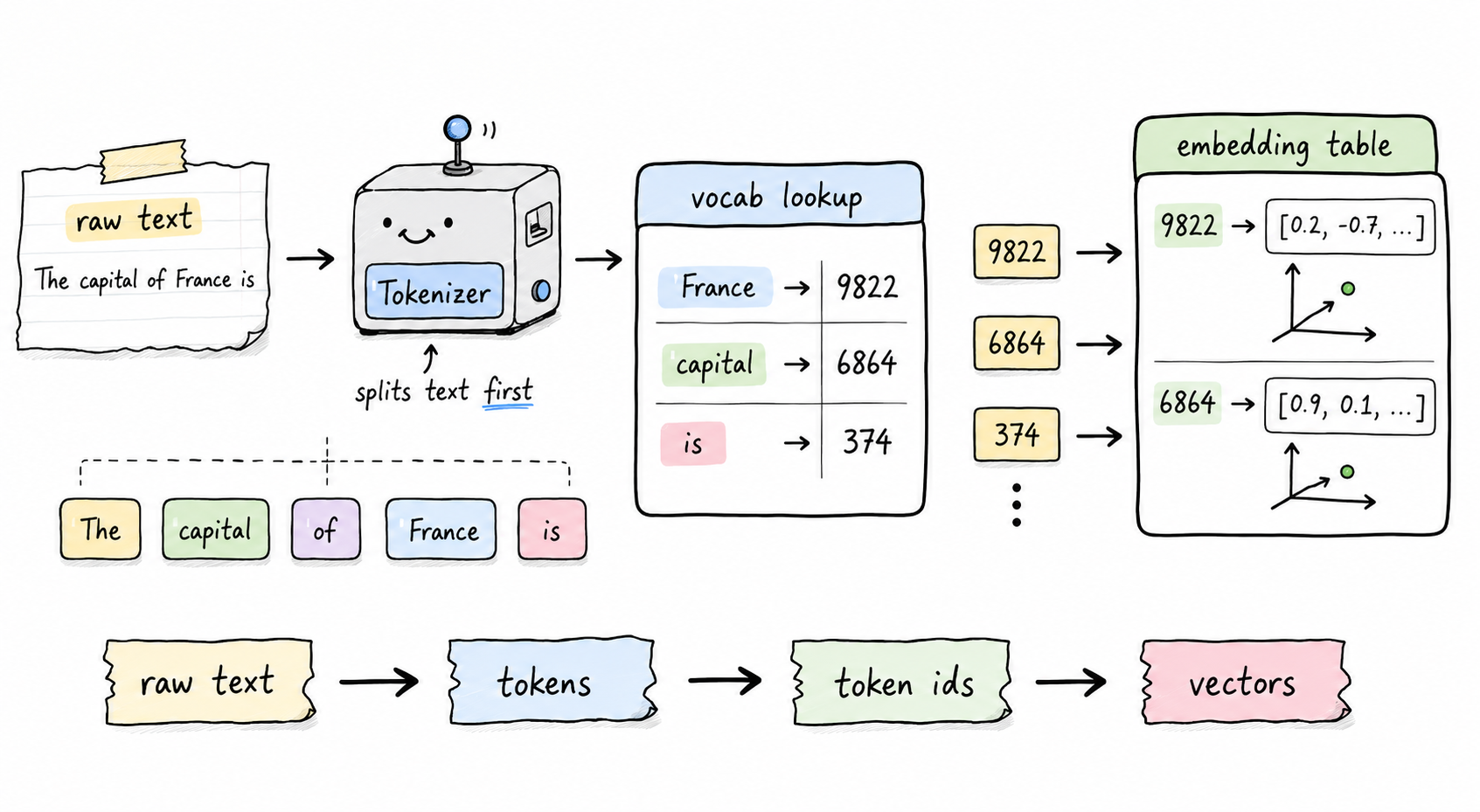
Tokenization means converting the text into the list of ids that the model knows how to process. So our prompt becomes something like [token_1, token_2, token_3, token_4, token_5]. The exact ids depend on the tokenizer, but what matters is the shape of the transformation:

text -> tokens -> token ids

Now token ids are still not enough. The model needs numbers it can do math on, so each token id is converted into a vector.

What Is A Vector Here?

A vector is just a list of numbers. A very tiny fake vector may look like this:

[0.12, -0.88, 1.41, 0.03]

Real LLM vectors are much bigger. They usually have thousands of dimensions, not 4. The model has an embedding table that knows how to convert each token id into a vector. So our sentence goes through this shape:

"The"      -> token id -> vector
" capital" -> token id -> vector
" of"      -> token id -> vector
" France"  -> token id -> vector
" is"      -> token id -> vector

Each token becomes a point in what’s called a vector space, a huge learned space where tokens with related meanings tend to be placed in related directions and regions.

For example, the token " France" starts with a rough meaning that sits near country-like things like Europe, the French language, Paris, maps, and national identity. The token " capital" starts near multiple possible meanings at once. It could be a city, a government, money, or an uppercase letter, depending on the context.

None of this is stored as English labels. The model doesn’t have a row somewhere saying "France" = country + Europe + Paris. It has numbers, and those numbers behave in a way where " France" is related to country-like things and " capital" is related to multiple possible meanings of capital.

So at the start, every token has a rough meaning and a point in that space.

There is one problem here. The position of a token, where it sits in the sentence, also matters, but the embedding table knows nothing about position. " capital" maps to the same starting vector whether it’s the first word of the prompt or the last.

But order is important. "The capital of France is" and "is France of capital The" use the exact same five tokens, just shuffled, and only one of them means anything.

To address this, the model adds the position directly into the token’s own vector, number by number. So the token’s vector now carries its meaning and its position at the same time, and any system that reads that vector later (like attention) has access to both automatically.

But the model doesn’t fully understand the sentence yet. That happens inside the layers.

The Transformer

Once the model has token vectors, it passes them through many transformer layers. A layer takes the current vectors and produces new vectors. After one layer, rough token vectors become slightly more contextual token vectors. After many layers, they become much richer contextual token vectors.

Back to our prompt. The vector for " capital" initially has multiple possible meanings like capital city, capital letter, financial capital, and capital punishment. Somewhere, the model has to settle on the capital city meaning. But the model doesn’t do this by rewriting the " capital" vector with information from " France". In GPT-style models, a token can only gather information from the tokens before it (we will see why in the causal mask section). " capital" only sees "The capital", so its vector sharpens a little, but it never sees " France".

The later tokens are where the sentence-level meaning builds up. The vector for " France" can see The capital of, so it stops being the standalone concept of France and becomes France, whose capital is being talked about. And the final " is" vector can see the whole prompt, so it becomes the place where capital + of + France combine into the capital city of France.

The model is not storing meaning as words. It is storing meaning as points and directions in a large learned vector space.

A transformer layer has two important pieces. Attention, which lets tokens gather information from other tokens, and a feed-forward network, which transforms each token vector further. Layer after layer, the vectors keep changing.

In simple words, a transformer is a giant vector-moving machine. It doesn’t look up "France" and return "Paris" from some table. It moves token vectors through learned transformations until the last token's vector strongly points toward a likely continuation.

We will come back to why the last token is important shortly

What Is A Weight?

We just used the term learned transformations. We also specifically mentioned the last token’s vector. Both of these details matter. First, let’s try to understand what learned transformations means.

A weight is a learned numeric setting inside the model. You can think of it like a tiny knob that controls how strongly one signal should affect another signal. If a signal should matter more, the learned settings strengthen it, and if it should matter less, they weaken it. In the real model, this happens by multiplying and combining the numbers inside vectors.

A model doesn’t have one giant bucket of a billion knobs where everything is mixed together. A billion-parameter model has billions of learned numbers, but those numbers are highly organized. They are stored in grids of numbers called matrices, and those matrices sit in specific parts of each transformer layer.

A transformer layer works more like an assembly line than one giant control panel. When a token vector enters a layer, it goes through a few stations in a fixed order.

First, it goes through the attention station. This part uses the attention block’s learned weights to create Queries, Keys, and Values. These are the pieces that let a token gather useful context from other tokens. We will talk about Queries, Keys, and Values properly in the next section. They will make more sense after we go through an example.

Then the enriched vector goes through the feed-forward station. This part uses a different group of learned weights to reshape the context-rich vector further.

Each station’s output gets added back onto the vector that was already there. So the attention station computes a correction and adds it on top of the incoming vector instead of replacing it. Same with the feed-forward station. This is usually called a residual connection (also called a skip connection).

A modern model can stack well over a hundred of these layers. If every layer fully replaced the vector, a small mistake early on would compound badly, and the token’s original identity could get lost somewhere around layer 40. Because each layer only adds a correction, the original signal survives the whole way through, and every layer only has to learn a small update instead of reconstructing everything from scratch.

After enough of this adding, the numbers inside the vector can drift into very large or very small ranges depending on what got added along the way. So each station also runs the vector through a quick normalization step before passing it on. This step checks how big the numbers have gotten and scales them back to a steady range. It doesn’t change what the vector means. It only keeps the math stable over so many layers.

Also, these stations don’t have the same number of knobs. In many transformer LLMs, the feed-forward part has more learned weights than the attention part.

The exact split depends on the model architecture, but the rough idea is that attention handles communication between tokens, and feed-forward does a lot of the per-token processing after that communication has happened.

So the token vector doesn’t touch all the knobs in the whole model at the same time. It moves through a sequence of learned transformations:

attention weights
-> feed-forward weights
-> next layer
-> attention weights
-> feed-forward weights
-> next layer

There are other details inside real transformer layers, but this is the useful mental model. The weights are partitioned by layer and by job.

The model is not carrying an English meaning like France = country + Europe + Paris when it applies these learned transformations.

It is carrying a long list of numbers, and as the vector moves through these organized blocks of weights, those numbers are changed. When those numbers change, what the vector represents also changes.

For our prompt, the weights are what decide that money, uppercase letters, and punishment don’t fit next to " of France", and that capital city does. The attention station can help the final " is" vector gather useful context from "The", " capital", " of", and " France".

The feed-forward station can then further reshape that context-rich vector so it points more strongly toward a likely continuation.

To be clear, there is no single knob called "Paris" or "capital city" anywhere. The knob is only a mental model. The real thing is a huge set of learned numeric settings, organized into different parts of the model, that together decide how vectors should be reshaped.

During training, the model learns these weights. During inference, when you are chatting with the model, those weights are fixed.

When you send a prompt to a normal LLM, you are not changing the model’s actual weights. You are only giving it context for this one generation.

How Attention Works

But how does a token know which other tokens to look at?

That’s where attention comes in. Attention is how tokens gather useful context from other tokens.

Here is our prompt again:

The capital of France is

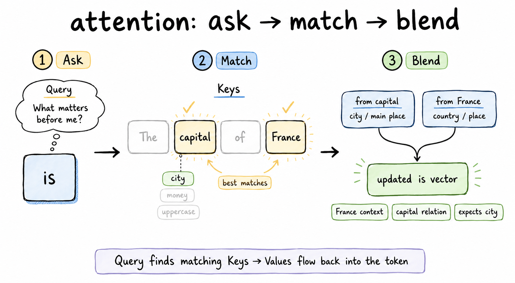
We said earlier that the vector for " capital" starts out ambiguous. It may mean a capital city, financial capital, or an uppercase letter. The model resolves this by letting later tokens look back at earlier tokens and gather their information. So let’s follow the final " is" token, the token that will eventually have to predict what comes next.

The common terms used in attention are Query, Key, and Value. These names sound more complicated than the idea. Roughly:

Query: what am I looking for?
Key: what kind of information do I have?
Value: what information can I share?

How Does A Token Become Query, Key, And Value?

When a token goes through attention, the model uses learned matrices to turn token vectors into three new vectors:

Query = what this token is looking for
Key   = what this token offers as a label
Value = what information this token can pass forward

Take our prompt, The capital of France is, and follow the token " is".

Step 1: Start With Token Vectors

Each token already has a vector, which is just a list of numbers. These vectors are the current internal representations of those tokens.

x_is      = vector for " is"
x_capital = vector for " capital"
x_france  = vector for " France"

Step 2: Create Query, Key, And Value

Inside the attention layer, the model has learned weight matrices W_Q, W_K, and W_V. These are grids of learned numbers. The model combines token vectors with these matrices:

q_is      = x_is * W_Q
k_france  = x_france * W_K
v_france  = x_france * W_V

This creates q_is (what " is" is looking for), k_france (what " France" advertises), and v_france (what " France" can contribute). The other previous tokens like "The", " capital", and " of" get their own Keys and Values in the same way.

W_Q, W_K, and W_V are different learned matrices, so they produce different versions of the same token vector. The same token can become a Query version, a Key version, and a Value version.

Step 3: Compare Query With Key

Now the model compares q_is with k_france using a dot product:

score = dot_product(q_is, k_france)

A dot product is basically a similarity score. If the Query from " is" matches the Key from " France" well, the score is high, which means " is" should pay attention to " France". If it doesn’t match well, the score is low, which means " France" is probably not very relevant to " is".

In the real model, " is" compares its Query against the Keys of many previous tokens. Then the scores are normalized, usually with softmax, so they become attention weights like:

The     -> 0.05
capital -> 0.40
of      -> 0.05
France  -> 0.50

Step 4: Use The Score To Pull Information

Now the model uses those scores to decide how much information to take from each token’s Value vector. If " France" gets a high score, its Value vector contributes a lot. If "The" gets a low score, its Value vector contributes only a little. Then the model adds these contributions together into one attention output. Conceptually:

attention output for " is"
=
0.05 * v_the
+ 0.40 * v_capital
+ 0.05 * v_of
+ 0.50 * v_france

So the " is" vector receives a lot of information from " capital" and " France".

Step 5: The Token Vector Gets Updated

That attention output is then used to update the current representation of " is". So " is" changes from a generic verb to something more like is, in a sentence asking for the capital city of France. In vector terms, the numbers inside the representation of " is" have changed, and because those numbers changed, what the vector represents also changed.

Step by step, that’s:

1. Create a Query for the current token.
2. Create Keys and Values for previous tokens.
3. Compare Query with Keys.
4. Use the match scores to blend the Values.
5. Update the current token vector with that blended information.

Attention uses learned weights to decide how tokens should pull information from other tokens: Query and Key decide the match, Value carries the information.

So the token " is" may create a Query like I am the point where the sentence continues, looking backward for what this sentence is about. The previous tokens present their Keys. "The" advertises determiner/article, " capital" advertises city/money/uppercase-letter, " of" advertises relation/possession, " France" advertises country/place/proper-noun. The Query from " is" compares with those Keys, and the best matches are " capital" and " France".

Then the model takes the Values from " capital" and " France" and blends that information into the vector for " is". So " is" no longer means a generic verb. It becomes something closer to is, expecting the capital city of France next.

The ambiguity of " capital" is gone here. On its own, the token could mean a city, money, or an uppercase letter. But when its information is blended with the information from " France" inside the " is" vector, the combination behaves like capital city of France. The money and uppercase-letter meanings simply don’t fit that combination, so they fade.

Attention is not one simple lookup. Every token can attend to many previous tokens, and the model has many attention heads, not just one (explained in more detail below).

One head may focus on grammar (which earlier words does this token depend on?), another may focus on meaning (which country is being talked about?), and another may focus on structure (which bracket or quote should match this one?). That’s why one token can be understood from many angles at the same time.

Attention Heads - More Context

When I first read about attention heads, my mental model was wrong. I thought one head means one match with one other token, and multiple heads exist so a token can match multiple tokens. Actually, a single head already compares one token against every previous token; multiple heads just mean the model runs that comparison several different learned ways at once as shown in the image below.

A head is one full attention system with its own Query, Key, and Value weight matrices. Inside one head:

1. Every token creates a Query
2. Every token creates a Key
3. Every token creates a Value
4. The current token's Query is compared against previous tokens' Keys
5. The matching scores decide how much of each previous token's Value to blend in

So even with one head, when the model is processing the final " is" in our prompt, it compares its Query against the Keys of "The", " capital", " of", and " France", gets a score for each, and blends their Values. The walkthrough we did above was exactly this, one head.

So what does multi-head attention add on top of this?

Instead of doing this once, the model does it many times in parallel. Each head has its own learned matrices:

Head 1: WQ1, WK1, WV1
Head 2: WQ2, WK2, WV2
Head 3: WQ3, WK3, WV3

Which means the same token vector becomes a different Query in each head:

q_is_head_1 = x_is * WQ1
q_is_head_2 = x_is * WQ2
q_is_head_3 = x_is * WQ3

For " is", the Queries may behave like:

Head 1: what is this sentence about?
Head 2: what type of token should come next?
Head 3: what grammar structure am I in?

The English words are our interpretation of the vector math, not something the model stores.

Each head then runs its own attention and lands on its own scores:

Head 1:
" is" attends mostly to " France"

Head 2:
" is" attends mostly to " capital"

Head 3:
" is" attends to nearby structure like "The" and " of"

Then all the head outputs are combined into one updated vector for " is". So one compact way to remember it is:

one head = one attention lens
many heads = many attention lenses

Each lens sees different relationships because each one has different learned weights.

Who decides how many heads?

Humans decide this when designing the model architecture, before training even starts:

token vector size = 4096
attention heads per layer = 32
each head works with 128 dimensions

So in a layer with 32 heads, a token gets 32 different attention lenses, 32 different learned query-types asked in parallel.

Who decides what the heads ask?

Training decides that. Nobody sits down and writes head 1 = grammar, head 2 = meaning. Each head starts with its own matrices, and during training the weights slowly adjust. Some heads end up becoming useful for certain patterns:

pronoun -> which noun does it refer to?
opening bracket -> where is the closing bracket?
adjective -> which word is it describing?
capital + country -> which relation is being completed?

This specialization happens on its own during training.

One more thing to note. A head’s question is a retrieval question. Attention asks which previous tokens should I read from? What to do with the gathered information is the feed-forward network’s job, which we will cover in the next section.

number of heads = chosen by the model designers
what each head learns to look for = learned during training
which tokens each head actually attends to = decided from the current prompt

Translated to English, attention is a token looking at the useful previous tokens and pulling their information into its own vector.

How Feed-Forward Works

Attention alone doesn’t explain everything. Feed-forward is a little harder to feel than attention, because attention has an obvious story: " is" looks back, finds " capital" and " France", and pulls information from them. There is no obvious story like that for feed-forward.

This was the part that took me the longest to internalize.

If attention asks which other tokens should I read from?, feed-forward asks what does this enriched vector now mean? That is the core idea.

In our prompt, after attention, the vector for " is" carries mixed signals. It is a linking verb, the sentence is about a capital, the country is France, a factual statement is being completed.

The feed-forward network works on this updated " is" vector and tries to reshape it into a better version for the next layer. It’s asking given these signals together, which learned features should become stronger?

For example, it may strengthen signals like the capital here means a city and not money, the expected next token is the name of a city, the city belongs to France. These are human descriptions for directions and signals inside the vector. The model itself has no English labels for any of this.

So the two do different jobs:

attention:
  moves information between tokens

feed-forward:
  processes the updated meaning inside each token

Attention mostly moves information around, like capital and France into is, or a function name into a later function call. Feed-forward processes the result. Capital + France means the likely answer type is a city, JSON key + value means this is structured data.

So a lot of the pattern processing happens inside feed-forward. Once the final " is" vector has gathered information from " capital" and " France" through attention, feed-forward can process that combined information and strengthen signals like “this is a factual completion”, “the relation is capital-of”, “the country is France”, “the expected answer is a city”, “Paris should become more likely” (again, directions inside the vector, not literal labels).

expand -> activate -> compress

before:
" is" = generic verb + pulled information from capital and France

after:
" is" = expecting the capital city of France next, ready for the next layer

Features, Signals, And Patterns

We have used words like features, signals, and patterns a few times now. These words are easy to mix up, so let’s make them more concrete.

A feature is a characteristic or a property. A signal is how strongly that feature is present. A pattern is a recognizable combination of signals.

So instead of thinking of a feature as a fixed object sitting somewhere inside the vector, think of it as a property that can be weakly or strongly active inside a vector. This distinction matters.

When I say the vector has a country signal or a city signal, I don’t mean there is a literal English label stored inside the model. I mean the numbers inside the vector are arranged in a way that behaves like that property is active.

Take our prompt again:

The capital of France is

After attention and feed-forward processing, the vector for " France" may carry a strong country signal, a strong Europe signal, and a strong capital-being-asked signal, alongside a weak person-name signal and a weak French-language signal.

The weak signals are also important. The model is not usually picking one clean box like this is only a country. It carries many possible properties at different strengths, and some of the weak ones may become useful later.

When multiple signals are active together, the model can recognize a larger pattern. Country + capital-of relation + factual completion adds up to the capital city of France, and that pattern can influence future tokens.

The model may make tokens like " Paris" much more likely, because the active pattern is the combination, the capital city of France, which is richer than capital or France alone.

This also connects back to the split between attention and feed-forward. Attention moves useful signals between token vectors. Feed-forward then checks, in a learned numeric way, which features are active, which combinations matter, and what should be written back into the vector.

So when we say feed-forward does pattern processing, this is the kind of thing we mean. It detects useful combinations of active signals and rewrites the token vector so the next layer has a better representation to work with.

Let’s put this together for the full prompt. The final " is" in The capital of France is has gathered information from all the previous tokens, so its vector may carry signals like:

factual-completion signal: strong
country signal: strong
capital-relation signal: strong
expects-city-next signal: strong
France-context signal: strong

Together, that pattern makes " Paris" score highly, because the current prompt activates a learned combination of signals that points strongly toward " Paris" as the next token. There’s no rule like if country == France and relation == capital: return Paris being executed anywhere.

When we say the model has “seen” a pattern before, we do not always mean it memorized that exact sentence. More accurately, during training the weights learn useful combinations of signals, and during inference the current prompt temporarily activates some of those combinations.

The Causal Mask

In GPT-style models, tokens are not allowed to see future tokens. This is called causal masking. For our prompt, the visibility roughly looks like this:

"The"      can see: "The"
"capital"  can see: "The", "capital"
"of"       can see: "The", "capital", "of"
"France"   can see: "The", "capital", "of", "France"
"is"       can see: "The", "capital", "of", "France", "is"

The first token doesn’t know the full sentence, but the last token does. This is why its final vector matters so much.

The model does not merge all token vectors into one big final vector and then predict from that. Instead, because of attention and causal masking, the last token’s vector becomes the place where useful previous context has been gathered.

For our prompt, the final vector at " is" becomes something like I have seen “The capital of France is”, the next token is probably a city name, and the city is probably Paris (a human description of what the vector represents, not literal stored text).

Predicting The Next Token

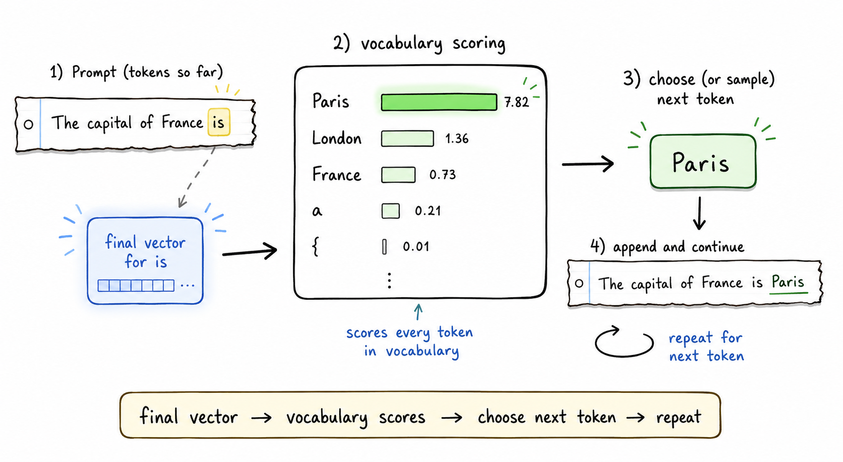
Now the model has a final vector for the last token. The next step is vocabulary scoring. The model has a fixed vocabulary, which is a menu of possible tokens like " Paris", " London", " the", " function", "{", and tens of thousands more.

The model takes the final vector of the last token and gives a score to every possible next token.

For our prompt, the scores may look roughly like:

" Paris"  -> very high
" London" -> lower
" France" -> lower
" a"      -> low
" {"      -> almost zero

Then it chooses or samples one token, and it emits Paris (more on how that choice actually happens further down). Now the text becomes The capital of France is Paris, and the model repeats the same process to predict the next token.

This is the generation loop:

take current text
turn it into tokens
convert tokens into vectors
move vectors through transformer layers
score the next token
choose one token
append it
repeat

That’s why LLMs stream text one piece at a time. There is no complete answer sitting inside the model waiting to be revealed slowly. The model is choosing the next token again and again.

Why It Can Be Wrong

The model scores likely next tokens. Nothing in this process verifies truth.

If the prompt points the model toward a wrong but plausible continuation, it may continue in that direction. For example, if the context strongly suggests a fake package name, fake API, or fake method, the model may produce something that looks very real.

The model is doing exactly what it was built to do, which is to produce a likely continuation for the given context. That continuation is often correct because the model has learned a lot of useful patterns. But likely and true are not the same thing.

This is also why hallucination is not some separate bug in the system. It comes directly from the same mechanism. If the model has no way to check the world, it can only continue from the prompt, the conversation so far, and the patterns stored in its weights.

That’s where retrieval, tools, and code execution come in. If the model can search your docs, query a database, inspect your repo, or run tests, then it is no longer only relying on what is inside its weights and current context. The base mechanism is still next-token prediction, but the context is now grounded in fresh external information.

Why Doesn’t It Always Pick The Best Match?

Back in Predicting The Next Token, we said the model “chooses or samples” one token from the score list. That word “or” actually covers two different strategies.

Before any picking happens, the model runs the raw scores through softmax. Softmax takes a list of scores and turns them into probabilities that add up to 100%, where a higher original score gets a higher share. Here it works on the scores for the model’s entire vocabulary, the same fixed list of possible tokens from Predicting The Next Token, and turns them into one probability distribution. Every token gets some probability, even " London" and " {". " Paris" simply gets most of it.

So does the model always pick the token with the highest probability?

Not always. Which strategy gets used changes how the model behaves.

Greedy decoding always takes the single highest-probability token. For our prompt, that’s " Paris" on every run. Ask the same question a hundred times and you get the same answer each time.

Sampling picks randomly, but not with equal chance for every token. Tokens with a higher probability get picked more often. " Paris" still wins most of the time since its share of the probability is so large, but once in a while a lower-scored token like " France" or " the" gets picked instead. The vectors and the scores are identical in both runs. Only the random pick differs.

Most chat products you use day to day sample by default. That’s the main reason the same prompt can give you a different-sounding answer on two separate runs.

This surprised me when I first understood it. The model isn’t confused when it rephrases something on a second try. That’s sampling doing what it was configured to do.

How much randomness goes into that pick is controlled by a setting called temperature. A temperature close to zero makes sampling behave almost like greedy decoding, mostly deterministic, always picking the safest token. A higher temperature makes the model more willing to pick a token it’s less sure about.

temperature 0.2:
" Paris"  -> 0.98
" London" -> 0.01
" France" -> 0.01

temperature 1.0:
" Paris"  -> 0.82
" London" -> 0.09
" France" -> 0.06
" a"      -> 0.02
" {"      -> 0.01

temperature 1.5:
" Paris"  -> 0.55
" London" -> 0.20
" France" -> 0.15
" a"      -> 0.07
" {"      -> 0.03

Same model, same prompt, same underlying scores. Only the shape of the distribution changes.

Temperature isn’t the only knob either. Top-k keeps only the k highest-scored tokens before sampling. Top-p (nucleus sampling) keeps adding tokens until their combined probability crosses a threshold instead of using a fixed count. Both are different ways of cutting down the candidate tokens before the random pick happens.

This is also a different failure source than the one covered in Why It Can Be Wrong. When sampling lands on a lower-probability token, the model is not confused about the world. The random pick simply landed differently on a distribution the model computed correctly.

None of this changes what the model actually knows. The vectors, the layers, the weights, all of that stays exactly the same. Temperature and sampling only change how willing the model is to pick a less likely token once it has already computed the probabilities. Low or zero temperature tends to get used for code generation, function calling, and factual lookups, where you want the same answer every time. Brainstorming and creative writing usually run at a higher temperature, where getting different answers is useful.

Where Does Thinking Fit In?

Newer models come with a “thinking” or “extended thinking” mode, sometimes called reasoning, where the model writes out a chain of intermediate steps before it gives you the final answer. It looks like a new capability sitting on top of the model, but mechanically it is the same generation loop from Predicting The Next Token, used to produce some extra tokens before committing to the final answer.

Every token gets the same fixed amount of computation: one pass through the stack of layers. That works fine for The capital of France is, where one pass is enough to make " Paris" the obvious next token. But take a prompt like:

A train leaves at 3:15pm and the trip takes 2 hours
and 50 minutes. What time does it arrive?

There’s no single vector position where the answer appears after one pass through the layers. The model needs to add 2 hours and 50 minutes to 3:15pm, and that’s a small sequence of steps, not a single lookup.

So instead of jumping straight to a final answer token, the model generates a run of intermediate tokens first, something like 2 hours takes us to 5:15pm, then 50 minutes takes us to 6:05pm. Each of those tokens goes through the identical loop: embed, move through the layers, score the vocabulary, pick a token, append, repeat. Nothing about the architecture changes for them.

What these extra tokens give the model is more passes through the layers before it has to answer. And because of causal masking, every later token can attend back to everything generated so far, including these intermediate ones. So the token that finally writes " 6:05pm" is not only attending to the original question. It is also attending to " 5:15pm" and " 50 minutes". The thinking tokens become extra context sitting in front of the answer, built by the model itself instead of by the user’s prompt.

But why does that give a better answer and not only a longer one? A forward pass is always the same fixed number of layers, no matter how hard the question is. So if a problem needs more steps than the network has layers, one pass through the stack simply cannot compute it. Writing extra tokens is the only way to get more total passes applied to the problem, since every new token means another full trip through the whole stack of layers.

There’s another reason for it. Think about what happens without any thinking tokens. The model would have to compute the whole thing inside one vector. The vector for the final token would somehow have to encode 3:15pm + 2h50m = 6:05pm entirely by itself, across the fixed stack of layers, and it never writes 5:15pm down anywhere as an actual value. That intermediate number, if it exists at all, is some pattern buried inside the vector, and every next layer keeps reshaping that pattern further. Nothing checks it along the way. If one layer changes it slightly in the wrong direction, the next layer continues with that wrong version. There’s no going back to correct it.

Now compare that to what happens with thinking tokens. " 5:15pm" gets written out as a real token in the sequence. It sits at its own fixed position, and like every token, it gets its own Key and Value the moment it’s produced. So when the model later needs to compute " 6:05pm", it doesn’t have to trust that some internal vector silently carried 5:15pm correctly across however many layers are left. It can attend directly to the actual " 5:15pm" token and pull its Value, the same Query, Key, Value lookup from How Attention Works.

Whether you actually see these tokens depends on the product, not the architecture. Some systems show you the full chain, some summarize it, and some hide it entirely and only stream the final answer. Underneath, the mechanism is the same. Only the amount of output shown to you changes.

A model isn’t automatically good at this just because it can generate more tokens. It has to be trained to use that budget well, to check its own steps, notice a mistake, and try a different path instead of confidently continuing down a wrong one. That training is usually a separate stage on top of the base model, and it’s what turns “generate some extra tokens” into something that actually reaches the right answer more often.

What About KV Cache?

There is one performance detail that explains why generation is fast enough to be usable. When a model generates text, it predicts one token, appends it, predicts the next token, appends it, and so on.

Naively, the model would have to recompute all previous tokens every time it generates a new token. That would be expensive.

Causal masking gives us a useful property here:

Old tokens cannot see future tokens, so their attention data does not need to change when a new token is appended.

Suppose the prompt is The capital of France is. The first pass processes all prompt tokens once. This is often called the prefill phase. During this pass, the model saves the previous tokens’ Keys and Values at each layer. That saved memory is called the KV cache, a Key cache and a Value cache.

Now the model predicts Paris. To predict the token after "Paris", it doesn’t need to recompute everything from scratch. The old tokens (The, capital, of, France, is) already have their Key and Value data saved.

So the model mostly processes the newest token, while letting that newest token attend backward to the cached Keys and Values.

Old tokens have already done their work, so their attention information gets saved. When a new token comes in, it reuses that saved information instead of computing it again.

old tokens:
  already processed
  keys and values saved
  not recomputed

newest token:
  goes through the layers
  creates queries
  attends to cached keys and values
  becomes context-rich
  predicts the next token

KV cache does not make the model smarter. It makes generation faster.

The Full Flow

If we put everything together, an LLM generation step looks like this:

That is the core mechanism. The model does not execute a handwritten rule for The capital of France is. It moves vectors through learned transformations until the final " is" vector strongly points toward continuations like " Paris", and then " Paris" gets a high score from the vocabulary menu.

Thanks for reading.